A new crustal 3-D P-wave velocity model beneath NE Tibet is determined by jointly inverting 62,339 high-quality first P-wave and later PmP-wave arrival-time data from local earthquakes and seismic explosions. Resolution tests show that the use of the PmP data can effectively improve the resolution of crustal tomography, especially that of the middle-lower crust. Widespread but intermittent low-velocity anomalies are revealed in the lower crust beneath NE Tibet, and the Kunlun fault acts as a transfer structure. High-velocity zones are visible in most parts of the crust below the transition zones bordering the southwestern Ordos basin between 105°~106° E longitude. We think that they form an important transpressive boundary to absorb sinistral strike-slip and thrust faulting deformation, like a western frontline of the Ordos basin, which is compatible with the latest GPS observations in the region. Considering the tectonic features and deformation of the Liupanshan fault, we need to pay much attention to the seismic risk of the fault zone from now. Our results reveal different structural features of the major blocks and their boundary faults, indicating the complexity of the Cenozoic crustal deformation in NE Tibet that partitioned between steep strike-slip shear zones and thrust faults.
Table 1. Data sets used in this study.
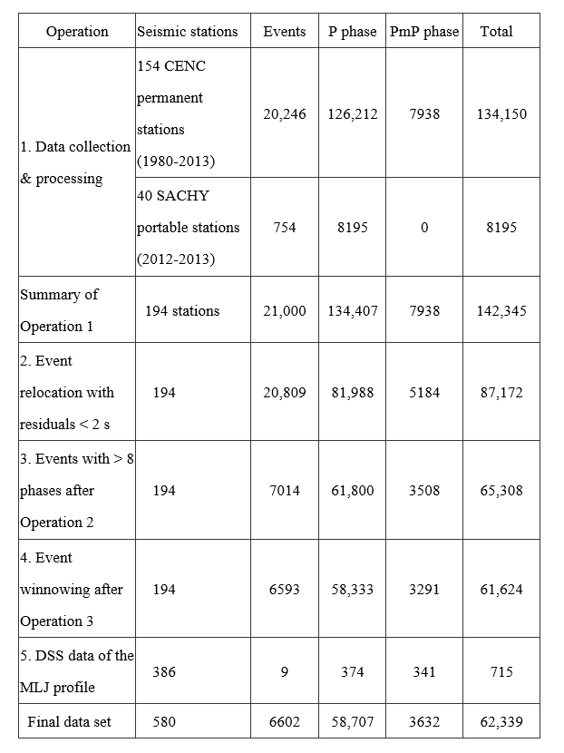
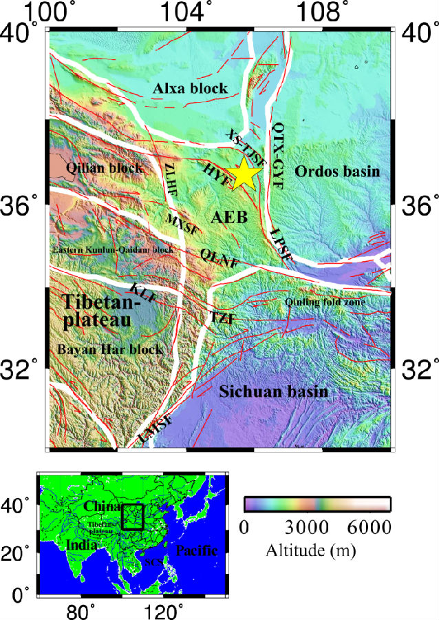
Figure 1. Tectonic background of the study region. The colors represent the surface topography whose scale is shown at the bottom-right. The inset map shows the location of the study region (black box) in Asia. The yellow star denotes the 1920 Haiyuan earthquake (M 8.5). The white thick lines denote boundaries of tectonic blocks (Deng et al. 2002; Zhang et al. 2003): the Alxa block (ALXB), the Ordos basin (ODB), the eastern tectonic belt of the Tibetan Plateau (AEB), the Qilian block (QLB), the Eastern Kunlun-Qaidam block (EKQB), the Bayan Har block (BYHB), the Qinling fold zone (QLFZ), and the Sichuan basin (SCB). The red lines denote active faults. The major faults are as follows (Lei & Zhao 2016; Ma 1989): the Longmenshan fault (LMSF), the Kunlun fault (KLF), the Tazang fault (TZF), the north Qinling fault (QLNF), the Zhuanlanghe fault (ZLHF), the Maxianshan fault (MXSF), the Liupanshan fault (LPSF), the Haiyuan fault (HYF), the Xiangshan-Tianjingshan fault (XS-TJSF), and the Qingtongxia-Guyuan fault (QTX-GYF).
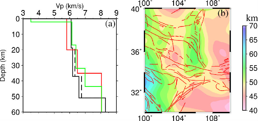
Figure 2. (a) The 1-D crustal P-wave velocity (Vp) models. The black dashed line denotes the LITHO1.0 model (Pasyanos et al. 2014), the black solid line shows a model modified from the LITHO1.0 model (the optimal 1-D model of the present study region), the red solid line shows the AK135 model, whereas the green line shows a model derived from the CRUST2.0 model. (b) The geometry of the Moho discontinuity in the study region derived from the LITHO1.0 model. The Moho depth scale is shown on the right. The red lines denote active faults.
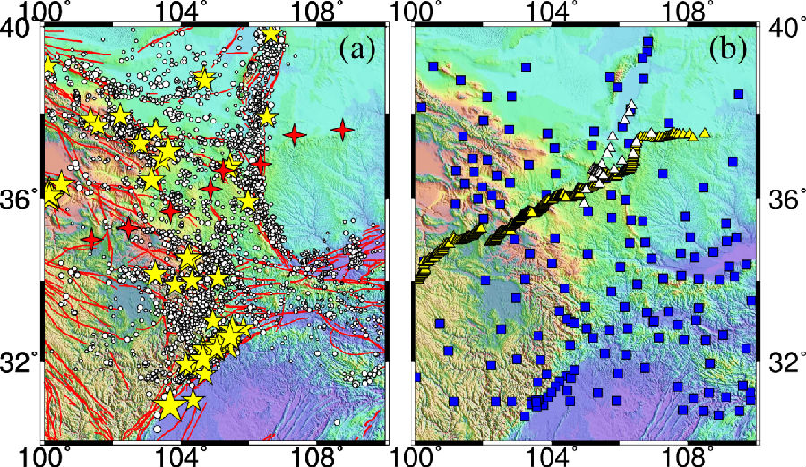
Figure 3. Distribution of the selected seismic events (a) and seismic stations (b) used in this study. In (a), the yellow stars denote earthquakes with magnitudes > 5.0 since 1980, whereas the white dots denote events < M 5.0. The red polar stars denote 9 shots in the deep seismic sounding experiment by the Research Center of Exploration Geophysics, China Earthquake Administration. In (b), the blue squares denote permanent seismic stations, the yellow triangles denote portable stations along the Maqin-Lanzhou-Jingbian (MLJ) profile deployed by Research Center of Exploration Geophysics, and the white triangles denote our SACHY array stations. The other labeling is the same as that in Figure 1.
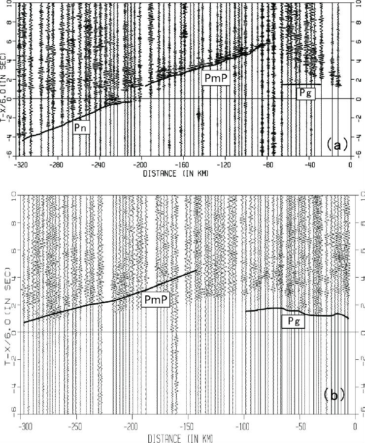
Figure 4. Reduced seismic record sections along the Maqin-Lanzhou-Jingbian (MLJ) refraction and wide-angle reflection profile (after Li et al. 2002). The seismograms were generated by the shots at (a) Jingbian (SP1032) and (b) Tongxin (SP800).
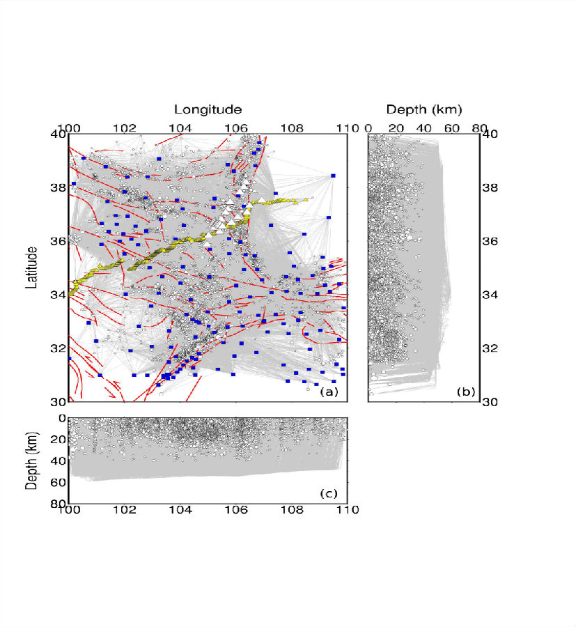
Figure 5. Distribution of ray paths (grey lines) from the 6602 seismic events (white dots) in the study area. Map view (a) and north-south (b) and east-west (c) vertical cross-sections. The blue squares and the white and yellow triangles denote seismic stations used in this study (see Figure 2b for details). The red lines denote the major active faults in the study region.
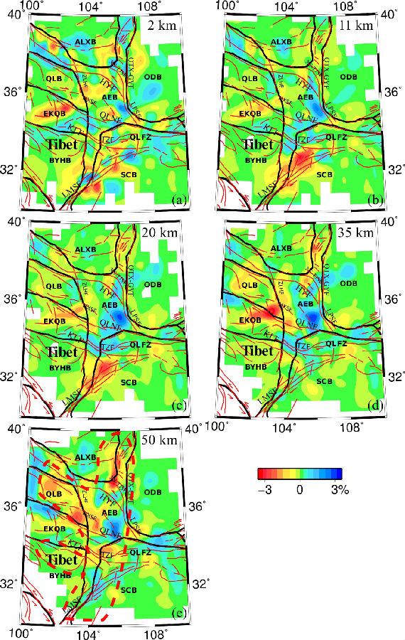
Figure 6. Map views of P-wave tomography obtained by a joint inversion of P and PmP wave arrival-time data. The layer depth is shown at the upper-right corner of each map. The red and blue colors denote low and high velocity perturbations, respectively, whose scale (in %) is shown at the bottom. The black lines denote boundaries of tectonic blocks. The red lines denote active faults.
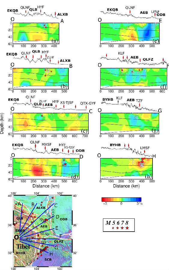
Figure 7. Vertical cross-sections of P-wave tomography along the eight profiles shown in the inset map. The three black lines in each section denote the Moho discontinuity and two other velocity boundaries in the crust. The red stars and black dots denote large earthquakes (M > 5.0) and smaller events (M < 5.0), respectively, within a 25 km width of each profile, which are all relocated using our new 3-D velocity model with more than 10 arrival-time data. The surface topography is shown above each cross-section. The red arrows denote the surface locations of major active faults. The other labeling is the same as that in Figure 1.
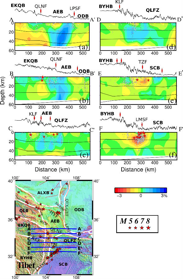
Figure 8. The same as Figure 7 but along the six profiles shown in the inset map.
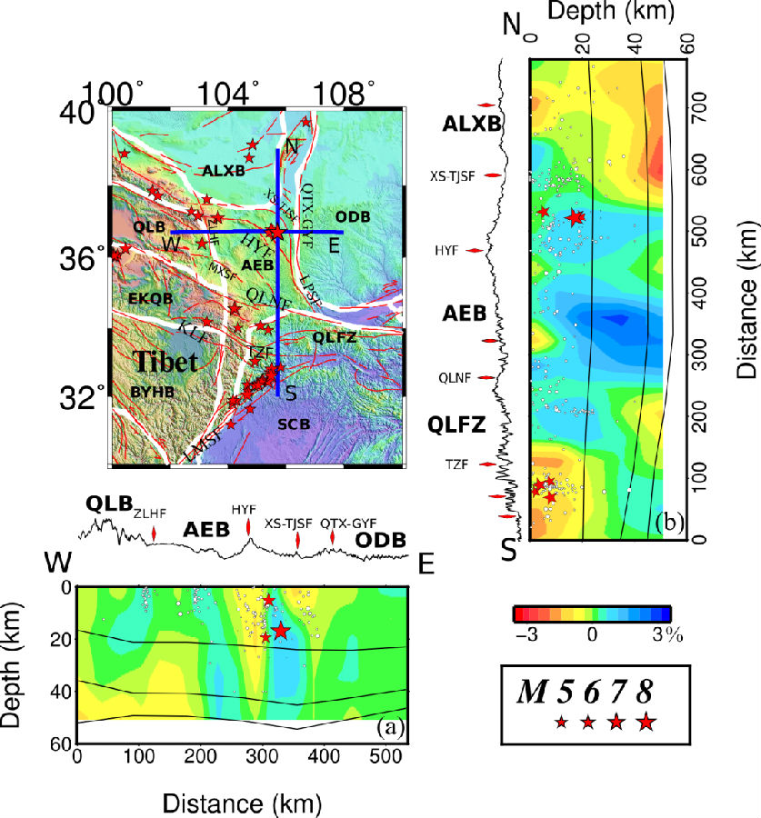
Figure 9. The same as Figure 7 but along the two profiles shown in the inset map, which pass through the epicenter of the 1920 Haiyuan earthquake (M 8.5; the biggest red star).
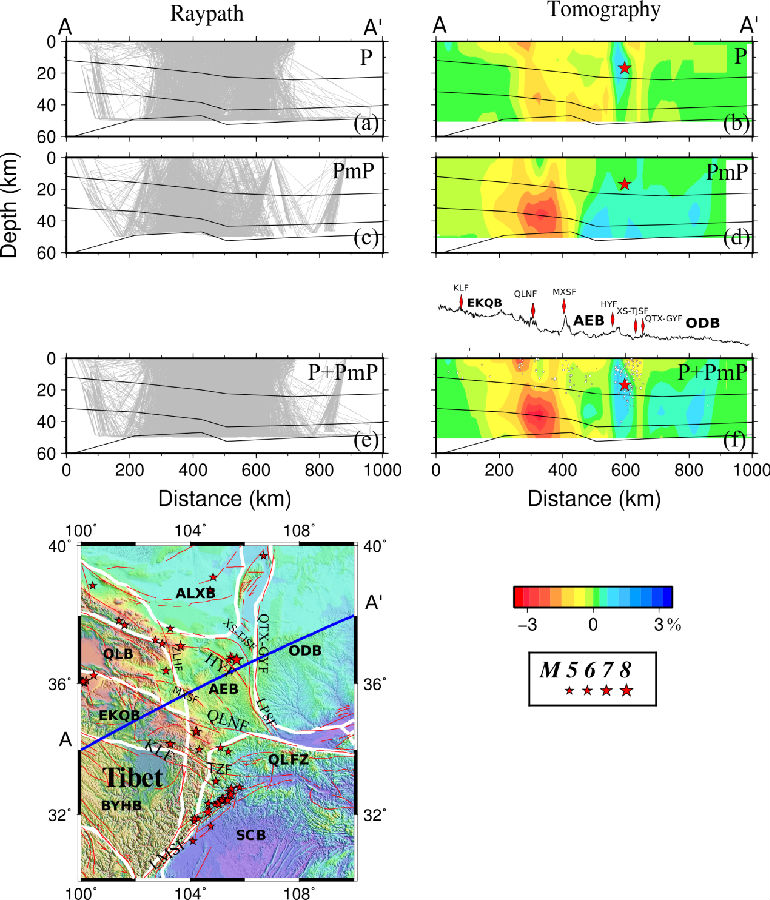
Figure 10. Vertical cross-sections showing the distributions of (a, c, e) ray paths within a 25 km width of the profile A-A’ and (b, d, f) P-wave tomography along the profile A-A’ as shown in the inset map. From the top to the bottom, the data used are the first P-wave arrivals (a, b), the PmP-wave arrivals (c, d), and both P and PmP arrivals (e, f), respectively. The other labeling is the same as that in Figure 7.
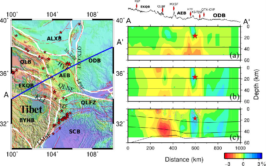
Figure 11. The same as Figure 10 but for P-wave tomography obtained by joint inversions of both the P and PmP data. The models in (a, b) are determined when flat velocity discontinuities are adopted. The model in (a) is obtained by inverting only the natural earthquake data. The model in (b) is obtained by inverting both the earthquake data and the DSS data. The model in (c) is the same as that in Figure 10f and is obtained using all the data and with curved velocity discontinuities.


